
There are hundreds of built-in functions in Microsoft Excel. Furthermore, you can use these functions together in different combinations to create powerful formulas. The ability to create formulas in Excel that solve complex problems is largely what makes the application so legendary. With that in mind, we will now look at 10 Excel functions that you should add to your repertoire.
IFERROR
The IF function is probably one of the most widely used functions among Excel pros. It is a logical function; if something is true then do something, otherwise do something else.
The ‘IF’ function allows you to build metadata – a set of data used to describe other data. Those same pros that use ‘IF’ also use the ‘IFERROR’ function to handle errors in their formulas.
We can use ‘IFERROR’ to specify an alternative value where a calculation might result in an error.
Let’s look at the ‘IFERROR’ function’s syntax:
There are two arguments in this formula: ‘value’ and ‘value-if-error’. The ‘value’ argument is the parameter the function tests for an error. This is most often another formula itself. Then the ‘value-if-error’ argument is the replacement value the user has selected for ‘IFERROR’ to return if the ‘value’ parameter does result in an effort.
The ‘value-if-error’ can be an actual static value such as a string or a number, but it can also itself be another formula. In the example that follows, we have an average price calculation in the ‘Average Price’ column. It is a simple division calculation that is susceptible to a divide by zero error (#DIV/0!).
In cell D6, this is precisely what has happened. However, by using the ‘IFERROR’ function, we can ensure that the value ‘0’ gets returned to the cell in the case of an error. Note the improvement to our result for row 6 in cell E6.

COUNTIF
Another popular ‘IF’ based function is ‘COUNTIF’. This function counts cells in a range where some specified condition is met. The syntax is simple. There are two arguments: ‘range’ and ‘criteria’. The ‘range’ argument is the range in which you are searching for the ‘criteria’. The ‘criteria’ argument is the specific condition that needs to be met for the count
=COUNTIF(range, criteria)
In the following example, we use ‘COUNTIF’ to count the number of employees by their years of service. Our ‘range’ argument is the column containing the ‘Year of Service’ for each employee, or “D2: D19” (the dollar signs preceding the column and row references are simply there to ‘lock’ the range for dragging the formula to other cells).
The ‘criteria’ argument is the years of service (1, 2 or 3). We could have placed the literal number values for ‘Years of Service’ as our ‘criteria’, but in this case, we opted to use the cell references for each (“F3”, “F4”, and “F5”, respectively). The ‘COUNTIF’ formula in each returns the count of employees corresponding to each value in ‘Years of Service’ in column G. Note the formulas for each row in column H.

CONCATENATE
The ‘CONCATENATE’ function is one of the most widely used in Excel. A point worth noting is that Microsoft introduced two new functions in Excel 2016 that will eventually replace ‘CONCATENATE’. They are ‘CONCAT’, a more flexible version of its predecessor, and ‘TEXTJOIN’. However, since not all Excel users have upgraded to Excel 2016, we will look at ‘CONCATENATE’.
The ‘CONCATENATE’ function combines strings of text and/or numerical values. Syntactically, this simply means placing the values you want to concatenate in sequential order, separated by commas. You can use either literal values or cell references as your arguments. You can use a combination of both as well.
=CONCATENATE(text1,[text2],…)
In the following example, we have two separate lists: first names and last names. Using the ‘CONCATENATE’ function, we will combine them in a column where we have the last name, then the first name separated by a comma. Then we can sort each by the last name in alphabetical order.

VLOOKUP
If you have spent much time with anyone with a reasonable amount of proficiency using Excel, you have likely heard of ‘VLOOKUP’. Like its sibling, ‘HLOOKUP’, it will search a table of values based on a criteria value.
The ‘VLOOKUP’ function will search the first column of a table for a criteria value and return a value from some specified number of columns to the right of that first column. The function consists of four arguments.
=VLOOKUP(lookup_value, table_array, col_index_number, [range_lookup])
The first argument is the ‘lookup_value’ is the value ‘VLOOKUP’ seeks a match for in the ‘table_array’ argument. In the following example, this is the cell reference ‘E2’ where we see the string ‘Finance’. We could have just as easily used the literal string ‘Finance’ as our ‘lookup_value’ argument. But using the cell reference allows us to change the value in ‘E2’ without changing the formula.
The ‘table_array’ is the table of values ‘VLOOKUP’ will seek a match for ‘Finance’ in the first column. Since our table is ‘A2: C7’, the match for our ‘lookup_value’ is on the first row (cell ‘A2’) of our ‘table_array’,
The ‘col_index_number’ argument is the number of the column from which we want ‘VLOOKUP’ to return a match on the same row from the ‘lookup_value’. In our case, we want ‘Average Years of Service’ in our formula in cell ‘F2’. This means we will insert ‘2’ as our ‘col_index_number’ argument since ‘Average Years of Service’ is the second column in our ‘table_array’.
The ‘range_lookup’ argument is an optional argument as denoted by the square brackets. This argument can be one of two values: TRUE or FALSE. A TRUE value tells the ‘VLOOKUP’ to return an approximate match while a FALSE value tells it to return an exact match. When omitted, the default for the formula is an approximate match.
In the following example, we can easily look up the average years of service and the average salary for employees by specifying the department.
An insider trick regarding ‘range_lookup’: try using ‘1’ and ‘0’ as a substitute for TRUE and FALSE, respectively. This is a shortcut that works just the same. Note in ‘G2’ our ‘VLOOKUP’ uses ‘0’ instead of FALSE.

INDEX And MATCH
The most basic example of what the ‘INDEX’ function does is that it takes an array, like a column of names. Then it takes a second argument, ‘row_num’, and returns the value from the array on that row.
=INDEX(array, row_num, [column_num])
Note that since we are working with a single column, we omit the optional ‘column_num’ argument since it is implied. However, if we were working with an array that had more than one column, we would use the ‘column_num’ argument in the same way we use the ‘row_num’ argument. ‘INDEX’ will return the value at the intersection of the two in the specified ‘array’.
In the following example, the ‘column_num’ is understood to be 1. This means the formula finds the value at the intersection of row 6 and column 1 of our ‘array’, ‘A2: A19’.

The ‘MATCH’ function takes a ‘lookup_value’, a ‘lookup_array’, and an optional ‘match_type’ argument. The ‘match_type’ argument allows for one of three values; ‘-1’ for less than, ‘0’ for an exact match, or ‘1’ for greater than.
=MATCH(lookup_value, lookup_array, [match_type])
In the next example, we pass in a string value for the ‘lookup_value’ and ‘0’ to ‘match_type’ for an exact match. See cell ‘C12’ for the result.
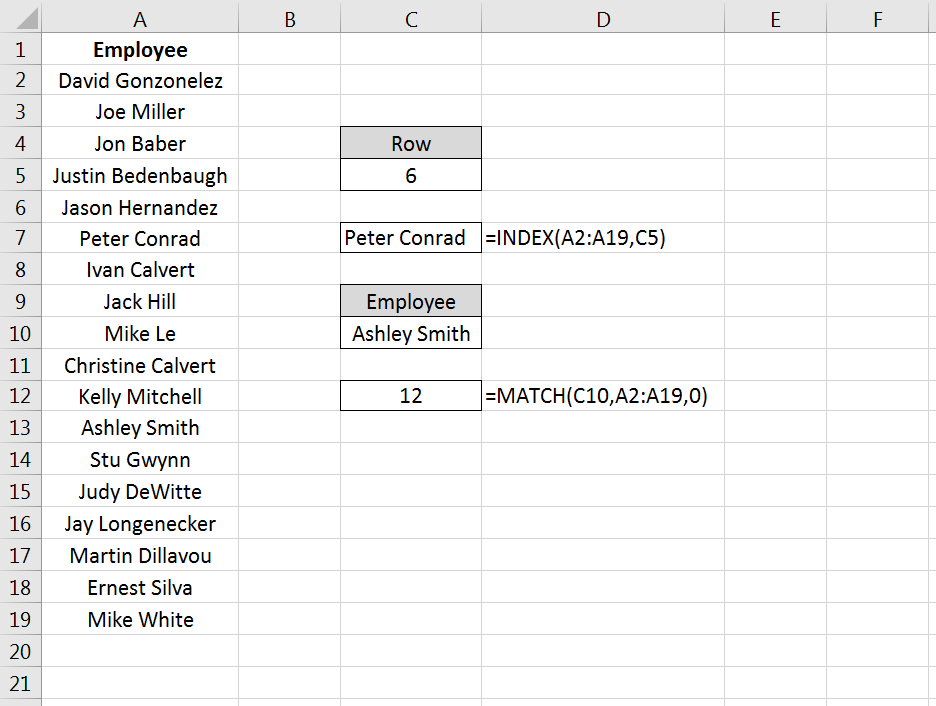
Now you have seen how you can find the row on which a value exists in a column using the ‘MATCH’ function. You have also seen how you can find the value in a cell by passing in a row number to the ‘INDEX’ function.
Imagine you had a second column with email addresses that you wanted to look up by employee name. See if you can figure out how to combine ‘INDEX’ with ‘MATCH’ to do just that. Hint: substitute the ‘MATCH’ formula for the ‘row_num’ argument in the ‘INDEX’ formula – then make sure you select the email column as the ‘array’ for your ‘INDEX’ function.
GETPIVOTDATA
This function is yet another type of lookup function but for Pivot Table users. It provides a direct method of retrieving tabulated data from Pivot Tables.
=GETPIVOTDATA(data_field ,pivot_table, [field1, item1], …)
The first argument, ‘data_field’, refers to the data field from which we want our result. In the following example, this will be our Pivot Table columns. The second argument, ‘pivot_table’, refers to the actual Pivot Table. In the following example, this is simply the cell reference ‘I3’, which is cell where our Pivot Table originates.
The third and fourth arguments, ‘field1’ and ‘item1’, refer to the field and row on which we want a match in the ‘data_field’. In our example below, our first ‘GETPIVOTDATA’ formula is looking for a match to the finance department in the ‘Average of Years of Service’ column.
Note that instead of hard-coding the literal value ‘Finance’ for the ‘item1’ argument, we have used the cell reference ‘N4’ where we have entered that string value. Just as we have seen with the other formulas we have covered, literal values or cell references can be used.

TEXTJOIN
We alluded to one of the newest functions in Excel, ‘TEXTJOIN’, in our earlier discussion about ‘CONCATENATE’. This function is only available in Excel 2016 desktop or in Excel online as a part of Microsoft 365.
Recall that the ‘CONCATENATE’ function requires an individual cell reference for each string. However, the ‘TEXTJOIN’ function allows you to combine strings by referring to multiple cells in a range. Usage of the ‘TEXTJOIN’ function is simple. There are three arguments.
=TEXTJOIN(delimiter, ignore_empty, text1, …)
The first argument, ‘delimiter’, is any string you want to be placed between the joined elements. This could be a symbol like a comma(“,”), or it could be a space (“ “). If you want nothing between the string elements you are joining, you still must specify that with the ‘delimiter’ argument. You simply insert two double quotes with nothing in between (“”).
The second argument, ‘ignore_empty’, allows you to tell the function whether you want to skip over empty cells when joining their values. This is simply a TRUE value for ignoring blanks, or FALSE when you do not want to ignore blanks.
The ‘text1’ argument is simply the cell or range of values you want to join. One thing to note is that you can add multiple ‘text’ arguments for each cell or range you want to be a part of the ‘TEXTJOIN’ formula.

Notice that we have a few blank cells in our range “A2: A19” but since we chose TRUE for the ‘ignore_empty’ argument, our result in the merged range “C2: G10” indicates no missing values between any of the commas.
FORMULATEXT
The ‘FORMULATEXT’ function returns the formula for a specific cell reference. If a formula is not present, the error value ‘#N/A’ results. This function provides an alternative way to visualize the formula present in a cell.
The syntax is incredibly simple:
=FORMULATEXT(reference)
The single argument, ‘reference’, is the cell reference where the formula exists. In the following example, there are multiplication formulas in column C. Placing a ‘FORMULATEXT’ function in the D column that references the cells on the same row in C, we can now visualize the formula as well as the result.

IFS
Another of the new functions available with Excel 2016 and Excel Online is the ‘IFS’ function. This function works in similar fashion as the ‘IF’ function, but it goes further by providing an efficient method of incorporating multiple logical tests and multiple values. Where in the past the same results would require nested ‘IF’ functions, the ‘IFS’ simplifies this process.
=IFS(logical_test1, value_if_true1, …)
In this example, we can assign a description of performance without utilizing nested IF statements.

Download Sample File
With the hundreds of available built-in functions with which to build your own formulas with, this list is by no means comprehensive. Furthermore, some of the functions on this list may not even resonate with your needs.
However, we curated the list with broad appeal in mind and feel that most Excel users could find a way to leverage these at some point. Sometimes the simplest functions lead to formulas that create great value. Moreover, sometimes it is difficult to know what is possible until you see them in action. We hope you find this list helpful and inspiring!